<?xml version="1.0" encoding="utf-8"?><feed xmlns="http://www.w3.org/2005/Atom" ><generator uri="https://jekyllrb.com/" version="3.10.0">Jekyll</generator><link href="https://aananthv.github.io/feed.xml" rel="self" type="application/atom+xml" /><link href="https://aananthv.github.io/" rel="alternate" type="text/html" /><updated>2026-06-06T10:12:15+00:00</updated><id>https://aananthv.github.io/feed.xml</id><title type="html">Aananth’s Blog</title><subtitle>Welcome to my personal blog. Here I share my thoughts, projects, and experiences working with technology, code, and everything in between.</subtitle><entry><title type="html">How LLMs Work - Part 1: Attention</title><link href="https://aananthv.github.io/machine/learning/2026/06/06/attention.html" rel="alternate" type="text/html" title="How LLMs Work - Part 1: Attention" /><published>2026-06-06T00:00:00+00:00</published><updated>2026-06-06T00:00:00+00:00</updated><id>https://aananthv.github.io/machine/learning/2026/06/06/attention</id><content type="html" xml:base="https://aananthv.github.io/machine/learning/2026/06/06/attention.html"><![CDATA[<h2 id="writing-an-llm-from-scratch">Writing an LLM from “scratch”</h2>

<p>Recently, I found myself becoming a “script kiddie” by following HuggingFace tutorials to try and post-train models. With the advent of coding agents, it has unfortunately become easier than ever to implement something without understanding what is happening under the hood. I am writing these (manually typed) notes to further my understanding.</p>

<h3 id="a-quick-digression-on-the-occams-razor">A quick digression on the Occam’s Razor</h3>

<p>While we may not be able to perfectly model the behavior and state of a <a href="https://en.wikipedia.org/wiki/Chaos_theory">chaotic</a> system, we should be able to define the set of constraints that govern the system. And, almost all of the chaos in the universe is governed by a set of simple, symetrical laws.</p>

<p>I firmly believe (albeit without proof) that the same must apply to the building blocks of life, consciousness, and intelligence (biological or otherwise). As an extension to the <a href="http://www.incompleteideas.net/IncIdeas/BitterLesson.html">Bitter Lesson</a>, I would bet that the algorithm that would eventually create general intelligence must be simple, easy to understand and easy to implement. Throughout these notes, I will only be discussing the algorithms that follow these principles.</p>

<h3 id="the-elegance-of-neural-attention">The Elegance of Neural Attention</h3>

<h4 id="fundamentals">Fundamentals</h4>

<p>Quoting <a href="https://en.wikipedia.org/wiki/Attention">Wikipedia</a>:</p>

<blockquote>
  <p>Attention is the concentration of awareness directed at some task or phenomenon while mostly excluding others.</p>
</blockquote>

<p>Given a collection of input signals, how can a neural network learn to direct its focus on the relevant signals?</p>

<p>Consider that we represent signals in an abstract vector space with $N$ dimensions:</p>

\[S_1 = (x_1, x_2, \dots, x_N)\]

\[S_2 = (y_1, y_2, \dots, y_N)\]

<p>To figure out how related these signals are, we can compute their similarity.</p>

<p>While we could use cosine similarity (calculated as $\frac{S_1 \cdot S_2}{|S_1| |S_2|}$) neural networks typically use the raw <strong>dot product</strong> for efficiency. Geometrically, the dot product measures how much two vectors align or point in the same direction, essentially capturing the overlapping “footprint” of one signal projected onto another.</p>

\[\text{Similarity} = S_1 \cdot S_2\]

<p>Given a set of signals $S_1, S_2, \dots, S_M$, we can efficiently compute the pairwise attention scores between all the signals using matrix multiplication.</p>

<p>If we stack the $M$ signals into an $M \times N$ matrix called $S$, we can compute:</p>

\[D = S S^T\]

<p>Let’s build an intuition of what this matrix $D$ signifies. $D$ is an $M \times M$ matrix, and each element $D_{ij}$ represents how similar $S_i$ and $S_j$ are. Ultimately, it tells us how much “attention” signal $S_i$ must pay to signal $S_j$.</p>

<p>Next, we normalize these attention scores by performing a softmax operation so that the sum of the attention scores for any particular vector is exactly 1.</p>

\[A = \text{softmax}\left(\frac{S S^T}{\sqrt{N}}\right)\]

<p>Notice that we scale the $D$ matrix by dividing it by $\sqrt{N}$ (the square root of the dimensions). We do this because large dot products can push the softmax function into unstable regions with extremely low gradients, which stalls the learning process.</p>

<p>We can then pull in the contributions of each signal $S_j$ into $S_i$ by computing a new composite signal, $O_i$, which is a weighted sum of all signals based on their attention scores:</p>

\[O_i = \sum_{j} A_{ij} S_j\]

<p>Using matrix multiplication once again to calculate this for all signals simultaneously, we arrive at our final output matrix:</p>

\[O = \text{softmax}\left(\frac{S S^T}{\sqrt{N}}\right) S\]

<p>If the $S$ matrix represents signals in isolation, and the $A$ matrix represents the instructions on who should listen to whom, the $O$ matrix represents the fully contextualized signals. Each row of O represents a contextualized version of the corresponding row in S.</p>

<p>Elegant, isn’t it?</p>

<h4 id="queries-and-keys">Queries and Keys</h4>

<p>Until now, a signal was comparing itself directly to other raw signals using $S S^T$. There is a teeny tiny issue with this approach: It assumes that “what a word is” is exactly the same as “what a word is looking for.”</p>

<p>If we compared raw signal values, we would always end up with the highest Dot Product for the same signal. Take the following phrase:</p>

<blockquote>
  <p>The heavy box fell on the fragile table, and <strong>it</strong> crushed <strong>it</strong></p>
</blockquote>

<p>If we compared the raw signal values of the second “<strong>it</strong>”, it would show highest similarity to the first “<strong>it</strong>”. However, we want each “<strong>it</strong>” to <em>attend</em> to a corresponding noun (“box”, “table”).</p>

<p>To make the network truly powerful, we want it to actively <em>learn</em> how to direct its attention. We do this by projecting our raw signals into a query dimentsion using learnable weight matrices: $W_Q$ and $W_K$.</p>

<p>When we multiply our input matrix $S$ by these weights, we generate new matrices:</p>

\[Q = S W_Q\]

\[K = S W_K\]

<p>These stand for <strong>Queries</strong> and <strong>Keys</strong>. The easiest way to build intuition for this is through a retrieval system:</p>

<ul>
  <li><strong>The Query ($Q$):</strong> This is what a signal is <em>looking for</em>.</li>
  <li><strong>The Key ($K$):</strong> This is what the signal <em>represents</em>.</li>
</ul>

<p>If we do this for our original sentence, the Query for the “<strong>it</strong>” might map it to a latent vector corresponding to <em>noun</em>. At the same time, Key vector will also map the nouns in the sentence to the same region. This makes the Attention mechanism serve more like a latent retreival than a raw similarity comparison.</p>

<p>Rewriting some of our equations from before:</p>

\[\text{Attention Scores} = Q K^T\]

\[O = \text{softmax}\left(\frac{Q K^T}{\sqrt{d_k}}\right) S\]

<p><em>(Note: We scale by $\sqrt{d_k}$, which represents the dimension of the Key vectors, ensuring our softmax gradients remain stable).</em></p>

<p>Another advantage of the projection is that they allow us to compute the Attention Score in a latent space with a different (lower) cardinality than the original Signals. This can make our computation faster!</p>

<h4 id="values">Values</h4>

<p>Currently, we calculated the Output matrix by multiplying the Attention Scores with the raw signals. While this would work in theory, we can do better. Consider the following sentence:</p>

<blockquote>
  <p>She matched her new <strong>paint</strong> to the sweet <strong>apple</strong> she was eating.</p>
</blockquote>

<p>Assuming the attention scores between “<strong>paint</strong>” and “<strong>apple</strong>” are high, what would we want “<strong>apple</strong>” to contribute to “<strong>paint</strong>”? If our Key vector mapped “<strong>apple</strong>” to “<strong>color</strong>”, we would want that <em>aspect</em> of “<strong>apple</strong>” to contribute to the Output for “<strong>paint</strong>”. That is we would want a corresponding mapping from “<strong>apple</strong>” to “<strong>red</strong>”.</p>

<p>We achieve this corresponding mapping using another set of trainable weights $W_V$ and compute the <em>Value</em> Matrix ($V$) as</p>

\[V = S W_V\]

<p>Substituting $Q$, $K$, and $V$ into our previous formula, we arrive at:</p>

\[O = \text{softmax}\left(\frac{Q K^T}{\sqrt{d_k}}\right) V\]

<p><em>(Note: $V$ needs to be the same dimensions as $S$ to satisfy the equation above, but this is not always a requirement).</em></p>

<p>By separating the inputs into Queries, Keys, and Values, the network is no longer just calculating blind similarity. It has learnable parameters that allow it to actively ask questions, advertise its own contents, and selectively share information across the sequence.</p>

<p>This exact mechanism, formally known as <strong>Scaled Dot-Product Attention</strong>, was introduced in the now ubiquitous “Attention Is All You Need” paper. By allowing networks to efficiently weigh the importance of different inputs, this mathematical operation became the foundation of the modern Transformer architecture.</p>

<h4 id="multi-head-attention">Multi Head Attention</h4>

<p>Consider the same sentence as before</p>

<blockquote>
  <p>She matched her new <strong>paint</strong> to the sweet <strong>apple</strong> she was <strong>eating</strong>.</p>
</blockquote>

<p>The <strong>Scaled Dot-Product Attention</strong> we described is perfectly capable of computing the Contextualized Output for the word “<strong>paint</strong>” by computing a vector corresponding to the color “<strong>red</strong>”.</p>

<p>But a single word can convey more information! In the same sentence, what if we want to compute the output score for the word “<strong>eating</strong>”? In this case, we can imagine that the Key for “<strong>apple</strong>” must correspond to something like “<strong>food</strong>” and the corresponding value must represent the “<strong>apple</strong>” itself.</p>

<p>We achieve this by having different sets of trainable weights $W_Q^i$, $W_K^i$, $W_V^i$ that “specialize” in extracting a different <em>aspect</em> of the input signal.</p>

<p>Subsituting into the earlier equations,</p>

\[Q_i = S W_Q^i\]

\[K_i = S W_K^i\]

\[V_i = S W_V^i\]

\[\text{Attention Scores}(i) = Q_i K_i^T\]

\[\text{head}_i = \text{softmax}\left(\frac{Q_i K_i^T}{\sqrt{d_k}}\right) V_i\]

<p>$\text{head}_i$ is the output of a single <strong><em>Attention Head</em></strong>.</p>

<p>Once all the heads have done their specialized extractions, their outputs are concatenated (glued together) and passed through one final weight matrix ($W_O$) to blend the insights of the entire committee back together into a single, incredibly rich contextual signal.</p>

\[O = \text{Concat}(\text{head}_1, \text{head}_2, ..., \text{head}_H)W_O\]

<p>Usually, to keep the amount of compute roughly constant, we make the dimension of each head:</p>

\[d_{head} = N / H\]

<p><em>(Note: Recall that $V_i$ need not be the same dimension as $S$)</em></p>

<p>By using multiple heads, the network doesn’t have to compromise. It can look at the word “apple” from 96 different perspectives simultaneously, extracting every nuance needed to understand the full picture.</p>]]></content><author><name></name></author><category term="machine" /><category term="learning" /><summary type="html"><![CDATA[Writing an LLM from “scratch”]]></summary></entry><entry><title type="html">RoPE and Local Attention hinder LLM performance</title><link href="https://aananthv.github.io/machine/learning/2025/05/03/rope-and-local-attention-hinder-llm-performance.html" rel="alternate" type="text/html" title="RoPE and Local Attention hinder LLM performance" /><published>2025-05-03T00:00:00+00:00</published><updated>2025-05-03T00:00:00+00:00</updated><id>https://aananthv.github.io/machine/learning/2025/05/03/rope-and-local-attention-hinder-llm-performance</id><content type="html" xml:base="https://aananthv.github.io/machine/learning/2025/05/03/rope-and-local-attention-hinder-llm-performance.html"><![CDATA[<h3 id="the-probability-of-answering-a-list-of-questions">The probability of answering a list of questions</h3>

<p>The <code class="language-plaintext highlighter-rouge">gemma-2-2b-it</code> model achieves a 56% score (5-shot)<sup id="fnref:gemma2" role="doc-noteref"><a href="#fn:gemma2" class="footnote" rel="footnote">1</a></sup> on the MMLU. <strong>What would we expect to happen if we asked it a batch of N questions at a time?</strong> In the ideal case, each of the questions would be answered correctly 56% of the time and this probability would simply be a independent variable that depends on the “intelligence” of the model.</p>

<p>However, this is not what we see!</p>

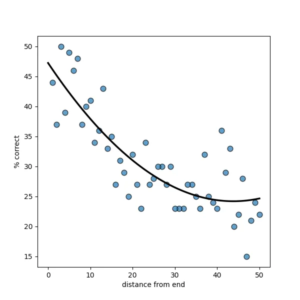
<p><img src="/images/rope/50.webp" alt="correct answers in batch of 50" /></p>

<p>When given a list of questions, the model gets the last question correct <strong>twice as often as the first question</strong>. The first few questions are pretty much guessed correctly with a random chance (25%).</p>

<p>Note: I ran these experiments using <code class="language-plaintext highlighter-rouge">gemma-2-2b-it</code> due to hardware limitations. Please try to run them on bigger models if you have the resources - I would love to see the results :)</p>

<h3 id="example-prompt">Example Prompt</h3>

<blockquote>
  <p>Read the following multiple choice questions and answer them one by one. Your answer for each question should be in following format: <question_number>. &lt;the index of the correct option (1, 2, 3, or 4)&gt;</question_number></p>

  <ol>
    <li>
      <p>Question: A family therapist using the structural approach of Salvador Minuchin would most likely:<br />
Choices:<br />
    1. clarify boundaries between family members in order to reduce enmeshment.<br />
    2. work initially with the most differentiated family member.<br />
    3. “use a multiple-therapist team to prevent any one therapist from becoming ““triangulated”” into the family system.”<br />
    4. “issue specific ““directives”” designed to counteract dysfunctional processes.”</p>
    </li>
    <li>
      <p>Question: Which of these countries was not a member of the Axis alliance during World War II?<br />
Choices:<br />
    1. Germany<br />
    2. Italy<br />
    3. Spain<br />
    4. Japan</p>
    </li>
  </ol>

  <p>(..the other questions, in a similar format)</p>

  <p>Here are the answers to the multiple-choice questions, one index per line:</p>
</blockquote>

<h3 id="pseudocode">Pseudocode</h3>

<p>The evaluation loop is fairly straightforward:</p>

<div class="language-py highlighter-rouge"><div class="highlight"><pre class="highlight"><code><span class="n">N_q</span> <span class="o">=</span> <span class="mi">50</span>      <span class="c1"># number of questions in a batch
</span><span class="n">N_iters</span> <span class="o">=</span> <span class="mi">100</span> <span class="c1"># number of iterations
</span>
<span class="n">scores</span> <span class="o">=</span> <span class="p">[</span><span class="mi">0</span> <span class="k">for</span> <span class="n">i</span> <span class="ow">in</span> <span class="mf">1.</span><span class="p">.</span><span class="n">N_iters</span><span class="p">]</span>
<span class="k">for</span> <span class="n">i</span> <span class="ow">in</span> <span class="mf">1.</span><span class="p">.</span><span class="n">N_iters</span><span class="p">:</span>
    <span class="c1"># batch is an array of size N_q containing (Q, A) tuples
</span>    <span class="n">batch</span> <span class="o">=</span> <span class="n">get_random_batch</span><span class="p">()</span>

    <span class="c1"># concatenate questions and add instructions for the model
</span>    <span class="n">prompt</span> <span class="o">=</span> <span class="n">format_prompt</span><span class="p">(</span><span class="n">batch</span><span class="p">)</span>

    <span class="c1"># generate output from the LLM
</span>    <span class="n">out</span> <span class="o">=</span> <span class="n">generate</span><span class="p">(</span><span class="n">prompt</span><span class="p">)</span>

    <span class="c1"># returns a boolean array
</span>    <span class="n">is_correct</span> <span class="o">=</span> <span class="n">check_answers</span><span class="p">(</span><span class="n">batch</span><span class="p">,</span> <span class="n">out</span><span class="p">)</span>
    
    <span class="c1"># scores[i] += 1 if is_correct[i]
</span>    <span class="n">update_scores</span><span class="p">(</span><span class="n">scores</span><span class="p">,</span> <span class="n">is_correct</span><span class="p">)</span>
</code></pre></div></div>

<h3 id="why-might-this-be-happening">Why might this be happening?</h3>

<p>I believe that there are two <em>optimizations</em> here that are bottlenecking LLM performance.</p>

<h4 id="1-local-attention">1. Local Attention</h4>

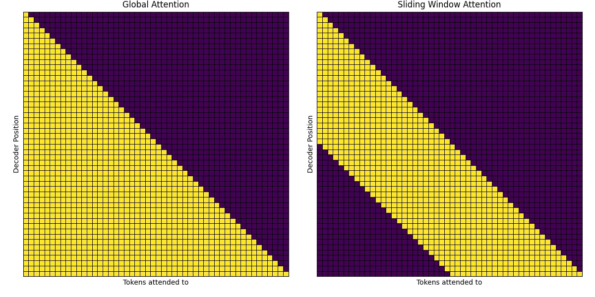
<p>Standard self-attention is powerful, letting every token “attend” to every other token in the context. However, this global view becomes computationally expensive (O(n^2)) as context length grows. Enter Local Attention<sup id="fnref:longformer" role="doc-noteref"><a href="#fn:longformer" class="footnote" rel="footnote">2</a></sup>. It’s an efficiency optimization technique. Instead of looking everywhere, each token only attends to a fixed-size window of its neighboring tokens. For decoder-only transformers like current LLMs, each token attends to a fixed-size window of preceeding tokens. This drastically reduces the computational cost (O(n)) and memory required, especially for long documents.</p>

<p><img src="/images/rope/sliding-window-1.webp" alt="sliding window attention" /></p>

<p>Gemma2 alternates between a 4096-token sliding window local attention layer and a global attention layer (8192 tokens, since that is the full context window). This interleaving allows the model to attend to the global state while being slightly computationally efficient.</p>

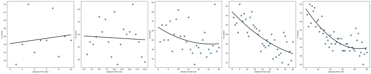
<p>This means that Gemma2 should be able to answer all the questions within the 4096-token window with the same accuracy. This seems to hold for the most part - when batches of &lt;20 questions are supplied, Gemma2 answers each question correctly with roughly the same probability.</p>

<p><img src="/images/rope/10-50-2.webp" alt="correct answers in batches of 10 to 50" /></p>

<p>However, I would imagine the graph to look more like a <a href="https://en.wikipedia.org/wiki/Heaviside_step_function">step-function</a> where questions within the 4096 context window are answered with probability P and the others are answered with a lower probability P’. This doesn’t seem to be happening - something else is causing the ~linear decrease in probability with distance within the 4096 sliding window.</p>

<h4 id="2-rope-rotary-positional-embedding">2. RoPE: Rotary Positional Embedding</h4>

<p>The attention mechanism is order-invariant, so it can’t distinguish <em>“boy eats sandwich”</em> from <em>“sandwich eats boy”</em> without positional information. This is generally performed by adding a <em>positional embedding</em> to the embedded tokens. Rotary Positional Embedding (RoPE)<sup id="fnref:rope" role="doc-noteref"><a href="#fn:rope" class="footnote" rel="footnote">3</a></sup> is used in pretty much all the SOTA open-source models including Gemma3, Llama4, and Qwen3. It is also used in Gemma2 - the model we’re testing. I found this <a href="https://youtu.be/o29P0Kpobz0?si=V0s7GqXxPk6nhrUB">youtube video by Efficient NLP</a> a great explanation of the different positional embeddings used in transformer architectures, including RoPE. RoPE also has advantages like context-window expansion, which makes it attractive for LLMs.</p>

<p>RoPE is applies a rotation to the Query (Q) and Key (K) vectors within the self-attention mechanism. The angle of rotation is determined by the token’s absolute position. The crucial insight is that when these rotated Q and K vectors interact via the dot product during attention calculation, the result naturally depends only on their relative distance.</p>

<p>However, since the attention between two tokens in a sequence is scaled by their dot product, RoPE causes a decay in attention between distant tokens. This is explained in the original paper that introduces RoPE as well.</p>

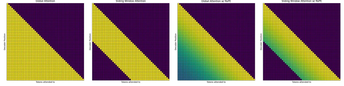
<p>For a simpler derivation, consider that tokens are represented in a 2d embedding space. To apply positional embedding, the token embeddings are rotated by some angle \(\theta = i\delta\) where \(i\) denotes the positon of the token in the sequence. It is clear that the dot-product between two <em>similar</em> embeddings spaced N tokens apart will scale by approximately \(\cos(N\delta)\).</p>

<p><img src="/images/rope/sliding-window-with-rope.webp" alt="sliding window attention with RoPE" /></p>

<p>This \(\cos(N\delta)\) decrease might explain the decrease within the 4096 sliding window.</p>

<h3 id="what-does-this-mean-for-llm-performance">What does this mean for LLM performance?</h3>

<p>A core assumption behind both of these optimizations is that <strong>most relevant context for predicting a token lies nearby</strong>. I imagine this is true for learning linguistic representations while pre-training LLMs to do next-token prediction, but does it still apply for the <strong>agentic tasks</strong> that we want these models to perform? I don’t think so. Agentic tasks generally do not differentiate between different parts of the context.</p>

<p>More recent architectures like Gemma3<sup id="fnref:gemma3" role="doc-noteref"><a href="#fn:gemma3" class="footnote" rel="footnote">4</a></sup> have both decreased the sliding token window to 1024 and decreased the frequency of the global attention layers to 1 in 5. While the Gemma3 paper reports no loss in perplexity due to this, I suspect the model will perform worse on this test. I wasn’t able to test on <code class="language-plaintext highlighter-rouge">gemma3-1b-it</code> because it wasn’t able to format the answers correctly according to the prompt (even when supplying just 1-2 questions) and the 4b+ models were too big to run.</p>

<p>While the open source world has not found any new alternatives to this issue, large labs might have. The Gemini models especially seem to support a 2M context window while simultaneously performing well on the <a href="https://cloud.google.com/blog/products/ai-machine-learning/the-needle-in-the-haystack-test-and-how-gemini-pro-solves-it">needle in the haystack test</a>. Regardless, this is certainly an important bottleneck that needs to be solved on the path to AGI.</p>

<hr />

<div class="footnotes" role="doc-endnotes">
  <ol>
    <li id="fn:gemma2" role="doc-endnote">
      <p>Gemma 2: Improving Open Language Models at a Practical Size. <a href="https://arxiv.org/abs/2408.00118">arXiv:2408.00118</a> <a href="#fnref:gemma2" class="reversefootnote" role="doc-backlink">&#8617;</a></p>
    </li>
    <li id="fn:longformer" role="doc-endnote">
      <p>Longformer: The Long-Document Transformer. <a href="https://arxiv.org/pdf/2004.05150">arXiv:2004.05150</a> <a href="#fnref:longformer" class="reversefootnote" role="doc-backlink">&#8617;</a></p>
    </li>
    <li id="fn:rope" role="doc-endnote">
      <p>RoFormer: Enhanced Transformer with Rotary Position Embedding. <a href="https://arxiv.org/abs/2104.09864">arXiv:2104.09864</a> <a href="#fnref:rope" class="reversefootnote" role="doc-backlink">&#8617;</a></p>
    </li>
    <li id="fn:gemma3" role="doc-endnote">
      <p>Gemma 3 Technical Report. <a href="https://arxiv.org/abs/2503.19786">arXiv:2503.19786</a> <a href="#fnref:gemma3" class="reversefootnote" role="doc-backlink">&#8617;</a></p>
    </li>
  </ol>
</div>]]></content><author><name></name></author><category term="machine" /><category term="learning" /><summary type="html"><![CDATA[The probability of answering a list of questions]]></summary></entry></feed>